
Methodology
Micrometeorological methods are widely recognized as providing the most accurate estimates of ammonia losses because they minimize the disturbance of environmental factors, such as wind speed and turbulence that affect ammonia volatilization (Denmead, 1983). The IHF system described below was established at three farms in central Montana, and one farm in southwest Montana.
Integrated Horizontal Flux - center mast approach
The IHF apparatus used in this study consists of a mast with five passive samplers or shuttles (Leuning et al., 1985) placed inside the center of circular plots. The radius of the plots is 20 m and the masts are situated 200 m apart (Figure 1).
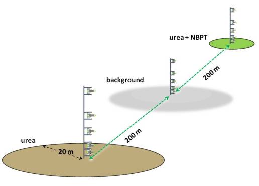
Figure 1. Field plot design used at the field sites. Masts are located in the center of circular plots within a field. Two plots are treated with urea and urea+NBPT (100 kg N/ha). The third mast is placed inside an unfertilized area to correct for background emissions.
The shuttles are arranged in a gradient spacing going up the mast (Figure 2). The center mast is approximately 3 meters high and is made of galvanized pipe. Each shuttle consists of a cone with an entrance hole, a PVC pipe cylinder with mounting pivots, and fins to keep the shuttle pointed into the wind (Figure 3). The interior of the shuttle contains a stainless steel spiral (Figure 4) which is coated with oxalic acid. During operation, air containing ammonia flows into the shuttle via the cone shape entrance hole and out an exit hole in the tail section. Once inside the shuttle the air is stripped of its ammonia by sorption to the spiral treated with oxalic acid.
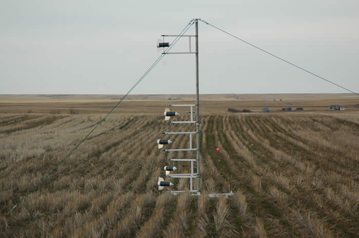
Figure 2. Masts in the center of circular plots hold five shuttles or samplers. Shuttles are placed at 0.25, 0.50, 1.0, 1.5, and 2.75 m above the soil surface.
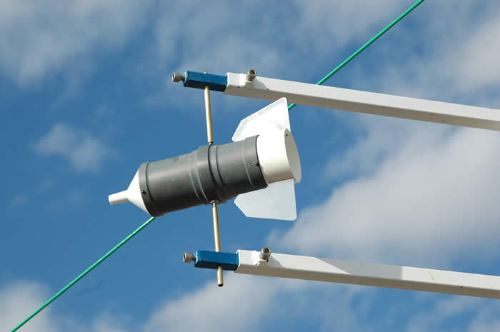
Figure 3. Shuttles pivot into the wind on two brass rods.
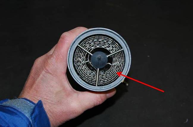
Figure 4: Close-up of shuttle with front cone removed showing interior stainless steel spiral.
Ammonia elution from shuttles, and analysis
Shuttles are exchanged approximately weekly. Spent shuttles are returned to the lab and the ammonia sorbed or precipitated on the stainless steel spiral is eluted in water. We place the shuttles between two end caps to form a sealed container (Figure 5). Deionized water (200 ml) is then added and the shuttle is rolled across the container top (Figure 6). The water or extract is transferred to a polyethylene bottle and ammonia is analyzed on a Timberline Ammonia Analyzer.
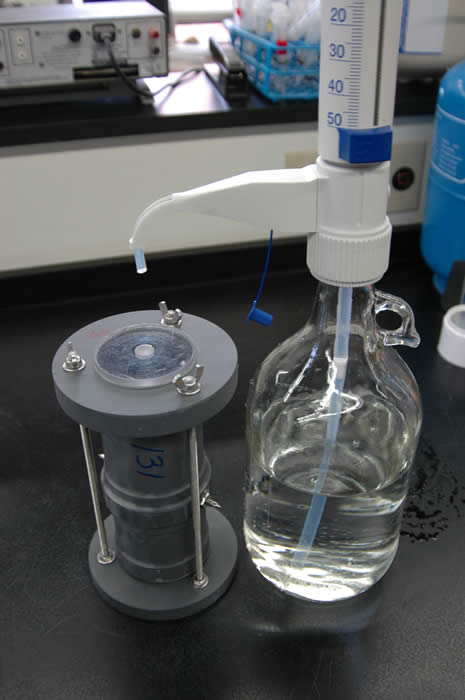
Figure 5. Water is added with a repipette through a hole in the top of the cap.
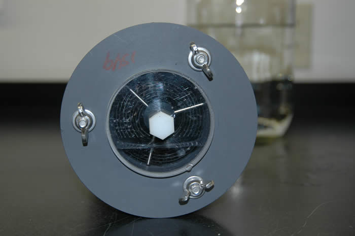
Figure 6. Shuttles are rolled across the counter-top, then shaken, to elute the ammonia trapped on the spiral.
Quantifying ammonia loss from fertilizer N
Step 1
Ammonia loss from fertilizer N is quantified by first calculating the horizontal flux in each of five planes and defined by the shuttle height above the ground (Figure 7). The horizontal flux for each of the five planes can be considered a time-integrated flux. The equation M/AT is used for this calculation; where M is the mass of ammonia-N sorbed by the shuttle and quantified during the elution and analysis phase (see subsection above), T is the time or sampling interval (our sampling interval is typically 7 days), and A is the effective sampling area of the shuttle.
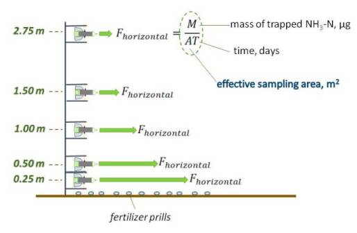
Figure 7. Horizontal ammonia-N flux is calculated at five heights or planes above the ground.
The effective sampling area of shuttle was defined in wind tunnel tests by Leuning et al. (1985). In these wind tunnel tests wind speed was varied while the air-flow rate through the shuttle was quantified. The relationship between the two variables was found to be linear (Figure 8). It is the slope of this line (=2.42 x 10⁻⁵ m2) that defines the effective sampling area or A. By defining the effective sampling area of the shuttle, Leuning et al. (1985) was able to eliminate the need to simultaneously measure wind speed (via anemometers) and gas concentrations at each height above the ground.
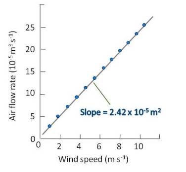
Figure 8. Wind speed tests conducted by Leuning et al. (1985) showed air flow through the shuttle varied linearly with wind speed. The slope of the line equals the shuttle's effective sampling area.
Step 2
The second step is to produce a scatter diagram of height above the ground vs. horizontal ammonia-N flux for each of the five planes. The area under the curve is then calculated (Figure 9).
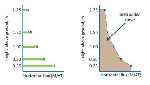
Figure 9. Scatter diagrams of height above ground vs. horizontal flux are created (left) and the area under the curve is calculated (right).
Step 3
Horizontal flux for each of the five heights is corrected for ambient ammonia by subtracting the horizontal flux from the background mast. The net area under the curve is then divided by the fetch distance (20 m in this study) to determine vertical ammonia-N flux (Figure 10).
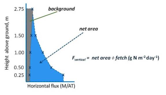
Figure 10. The area under the curve is corrected for background emissions of ammonia.
Step 4
Once vertical flux (Fv)has been calculated. The ammonia-N loss is quantified by multiplying Fv by the sampling interval or number of days the shuttles were left on the mast. In our study this is ~7 days. If we know the amount of ammonia-N loss we can calculate the fraction or percentage of fertilizer N lost over this sampling interval, by dividing by the fertilizer N rate (10 g m-2 or 100 kg N/ha).
Literature Cited
- Denmead, O.T. 1983. Micrometerological methods for measuring gaseous losses of nitrogen in the field. p. 131-157. In J.R. Freney and J.R. Simpson (eds.) Gaseous Loss of Nitrogen from Plant-Soil Systems Martinus Nijhoff Publishers: The Hague, Netherlands.
- Leuning, R., J.R. Freney, O.T. Denmead, and J.R. Simpson. 1985. A sampler for measuring atmospheric ammonia flux. Atmos. Environ. 19:1117-1124.